The regurgitate extension automatically collects all code blocks from your document and places them in a “Code Appendix” at the end. This is useful when you want readers to follow your narrative without hunting for code, while still providing complete source code for reproducibility.
Add the regurgitate filter to your document’s YAML front matter like so:
---title: "Sample Usage"filters: - regurgitate---
And voila! With no configuration, code appears both in its original location and in the appendix.
Computing Summary Statistics
Let’s compute some summary statistics using Python. We can see both the Python code and its output here.
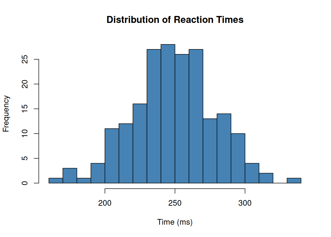
Similarly, we can create a histogram in R to visualize a distribution of reaction times.
# Generate sample data, create a histogram, and summarizeset.seed(42)reaction_times <-rnorm(200, mean =250, sd =30)hist(reaction_times, main ="Distribution of Reaction Times",xlab ="Time (ms)", col ="steelblue",breaks =15)
summary(reaction_times)
   Min. 1st Qu.  Median    Mean 3rd Qu.    Max.
  160.2   231.7   249.5   249.2   269.0   331.1
Conclusion
At the bottom of this page, you’ll find a Code Appendix containing both code blocks above, making it easy for readers to copy all code at once.
# Generate sample data, create a histogram, and summarizeset.seed(42)reaction_times <-rnorm(200, mean =250, sd =30)hist(reaction_times, main ="Distribution of Reaction Times",xlab ="Time (ms)", col ="steelblue",breaks =15)summary(reaction_times)
   Min. 1st Qu.  Median    Mean 3rd Qu.    Max.
  160.2   231.7   249.5   249.2   269.0   331.1